
Experimental Control for Machine Learning of Temporal Effects in Quantitative Trading

Experimental control is one of the foundational principles of sound scientific experimentation. Its importance lies in ensuring that the conclusions drawn from an experiment are valid and attributable to the factor(s) being investigated, rather than to confounding variables.
Experimental control allows researchers to manipulate only the independent variable(s), establishing causal relationships by controlling extraneous variables (through design, randomisation, or standardisation).
Let’s consider a humorous story:
Hanguk, a curious scientist decided to test out Johnson’s claim that Mlaetoinn increases nighttime erection length. He invited 10 male volunteers, and 10 female volunteers. The men consumed Mlaetoinn. The 10 men recorded an average nighttime erection of 1 hours, and the 10 women recorded 0 hours of erection.
He concluded that Mlaetoinn increases nightime erection length.
In trading, experimental design to validate and test trading strategies are not yet comprehensively understood, and there is no industry standard. Quoting from The Elements of Quantitative Investing;
…best practices for backtesting - They do not originate from some comprehensive theory. Unlike Athena, who was born fully formed from the mind of Zeus, it is an ever-incomplete, occasionally shallow body of knowledge that has formed by experimentation.
This post aims at discussing the construction of experimental control for financial data, with applications in statistical hypothesis testing. The ideas are largely based on permutation sampling, motivated by Masters, with original extensions and implementation in Python.
In permutation sampling, we aim to destroy local temporal structure in financial time series while preserving global statistical properties such as marginal distributions, moments of distribution like overall market drift.
This technique is particularly useful in statistical hypothesis testing: for example, to evaluate whether a trading strategy performs better than chance. By comparing strategy performance on real market data (where predictability may exist) against permuted data (where predictability is fully removed), we can assess the likelihood that observed performance arises from random chance.
Formally given a time series {x_t}, we apply a random permutation PI: [T] → [T] to obtain
where x_t denotes some stationary distribution. If only univariate values are permuted, the autocorrelation is destroyed, but the moments are preserved. In contrast, multivariate permutations (e.g., row-wise permutations of bar data) preserve cross-sectional structure and marginal distributions while eliminating temporal dependencies.
Even though synthetic data such as Brownian motion or Brownian bridges can be used to generate price paths, they introduce new assumptions and modify multiple statistical properties simultaneously. In scientific procedures, we aim to control all variables except the one under investigation — otherwise, conclusions are confounded by uncontrolled factors.
Permutation methods offer a principled alternative: they destroy temporal structure (and thus predictability) while preserving other features of the data. This makes them ideal for scientific experiments.
Univariate (Price) Permutations
In univariate permutation sampling, we focus on transforming a single price series — such as closing prices — by permuting its internal structure while preserving global properties such as overall trend.
Here, we seek a variant that preserves the initial and final price levels, ensuring the global drift remains intact. This is achieved by permuting the log returns (or equivalently, the log price differences), which are assumed to be approximately stationary, then reconstructing the price path via exponentiation.
Let {P_t} denote the original price series, then define the log returns:
We apply the permutation algorithm to {D_t}, obtaining a permuted seqeuence {D_t’}.
To generate a member of a permutation set
def permutation_member(array):
    i = len(array)
    while i > 1:
        j = int(np.random.uniform(0, 1) * i)
        if j >= i: j = i - 1
        i -= 1
        array[i], array[j] = array[j], array[i]
    return array
We then reconstruct the permuted log price path by cumulative summation:
and exponentiate the result to obtain the new permuted price series.
def permute_price(price):
    log_prices = np.log(price)
    diff_logs = log_prices[1:] - log_prices[:-1]
    diff_perm = permutation_member(diff_logs)
    cum_change = np.cumsum(diff_perm)
    new_log_prices = np.concatenate(([log_prices[0]], log_prices[0] + cum_change))
    new_prices = np.exp(new_log_prices)
    return new_prices

# Example usage
permuted_price = permute_price([3, 1, 2, 4, 5, 4, 6, 4])
print(permuted_price)
# [3.0000, 6.0000, 4.8000, 9.6000, 14.399, 4.8000, 3.2000, 4.0000]
This method preserves the first and last price, destroys temporal dependence, and retains the marginal distribution of log returns. It provides a robust null model for hypothesis testing when testing for time-dependent structure in univariate financial series.
When working with multiple price series from different instruments, we aim to preserve the inter-series structure (e.g., cross-instrument correlation) while eliminating only temporal dependencies.
Applying independent permutations to each price series destroys their joint distribution, including cross-asset dependencies and synchronized drawdowns. This can distort portfolio-level risk metrics and undermine hypothesis tests designed to isolate time-series predictability.
To address this, we generalize the permutation method by applying a single shared permutation index across all series. This preserves the joint distribution of returns across instruments while removing their individual serial structure.
def permute_price(price, permute_index=None):
    if permute_index is None:
        permute_index = permutation_member(list(range(len(price) - 1)))
    log_prices = np.log(price)
    diff_logs = log_prices[1:] - log_prices[:-1]
    diff_perm = diff_logs[permute_index]
    cum_change = np.cumsum(diff_perm)
    new_log_prices = np.concatenate(([log_prices[0]], log_prices[0] + cum_change))
    new_prices = np.exp(new_log_prices)
    return new_prices

def permute_multi_prices(prices):
    assert all(len(price) == len(prices[0]) for price in prices)
    permute_index = permutation_member(list(range(len(prices[0]) - 1)))
    new_prices = [permute_price(price, permute_index=permute_index) for price in prices]
    return new_prices
This shared-index approach ensures that all series undergo the same reordering of returns, thereby preserving inter-series alignment. It is suitable for evaluating the statistical significance of multi-instrument strategies, including long-short spreads, mean-reversion baskets, and cross-sectional alpha signals.
Multivariate (Bar) Permutations
In many practical settings, we work with multivariate time series data, such as OHLCV bars or engineered features per time step. Each time point t∈[T] is associated with a vector
where d denotes the number of features (e.g., open, high, low, close, volume, technical indicators, etc.).
Unlike univariate series, there is no universally accepted method for permuting multivariate data. Since such data often arise from dynamic systems with complex temporal and cross-feature dependencies, care must be taken to preserve internal structure while destroying serial correlations.
We illustrate this using OHLCV bars, also known as candlesticks. These may be constructed using time-based sampling or entropy-based sampling schemes such as information bars. Our key goal is to preserve bar-level structure (intra-bar) while eliminating time dependence (inter-bar).
Intra-bar structure. Each bar comprises price levels: open Ot, high Ht, low Lt, and close Ct. Rather than permuting absolute values, we first log-transform the prices and define:
These deltas characterize the internal geometry of each bar and remain approximately stationary after log-transformation.
Inter-bar structure. A natural candidate for inter-bar relationship is the jump between a bar's close and the next bar's open:
Volume data. Volume is particularly challenging to permute. It may be stationary or non-stationary depending on the asset and sampling method, and can exhibit strong periodic effects (e.g., time-of-day, day-of-week seasonality). Since volume interacts with both price levels and bar duration, careless permutation may distort the joint distribution of intra- and inter-bar features.
To implement the controlled permutation of multivariate OHLCV bars, the observe the following procedure:
Log-transform the OHLCV dataframe.
Compute the intra-bar differences ΔH, ΔL, ΔC.
Permute these intra-bar differences (excluding the first row) using a common permutation index.
Compute the inter-bar open-to-close jumps ΔOC(t) = O(t+1) − C(t) and permute them independently.
Reconstruct the full price path iteratively:
Start from the first close.
Add a (permuted) ΔOC(t) to compute each new open.
Add (permuted) intra-bar deltas to get the high, low, and close.
Volume is permuted alongside the intra-bar deltas, preserving the endpoints.
The resulting log-prices are exponentiated and reassembled into a new dataframe with the original index.
import numpy as np
import pandas as pd

def permute_bars(ohlcv, index_inter_bar=None, index_intra_bar=None):
    if not index_inter_bar:
        index_inter_bar = permutation_member(list(range(len(ohlcv) - 1)))
    if not index_intra_bar:
        index_intra_bar = permutation_member(list(range(len(ohlcv) - 2)))

    log_data = np.log(ohlcv)
    delta_h = log_data["high"].values - log_data["open"].values
    delta_l = log_data["low"].values - log_data["open"].values
    delta_c = log_data["close"].values - log_data["open"].values
    diff_deltas_h = np.concatenate((delta_h[1:-1][index_intra_bar], [delta_h[-1]]))
    diff_deltas_l = np.concatenate((delta_l[1:-1][index_intra_bar], [delta_l[-1]]))
    diff_deltas_c = np.concatenate((delta_c[1:-1][index_intra_bar], [delta_c[-1]]))

    new_volumes = np.concatenate(
        (
            [log_data["volume"].values[0]],
            log_data["volume"].values[1:-1][index_intra_bar],
            [log_data["volume"].values[-1]]
        )
    )

    inter_open_to_close = log_data["open"].values[1:] - log_data["close"].values[:-1]
    diff_inter_open_to_close = inter_open_to_close[index_inter_bar]

    new_opens, new_highs, new_lows, new_closes = \
        [log_data["open"].values[0]], \
        [log_data["high"].values[0]], \
        [log_data["low"].values[0]], \
        [log_data["close"].values[0]]

    last_close = new_closes[0]
    for i_delta_h, i_delta_l, i_delta_c, inter_otc in zip(
        diff_deltas_h, diff_deltas_l, diff_deltas_c, diff_inter_open_to_close
    ):
        new_open = last_close + inter_otc
        new_high = new_open + i_delta_h
        new_low = new_open + i_delta_l
        new_close = new_open + i_delta_c
        new_opens.append(new_open)
        new_highs.append(new_high)
        new_lows.append(new_low)
        new_closes.append(new_close)
        last_close = new_close

    new_df = pd.DataFrame(
        {
            "open": new_opens,
            "high": new_highs,
            "low": new_lows,
            "close": new_closes,
            "volume": new_volumes
        }
    )
    new_df = np.exp(new_df)
    new_df.index = ohlcv.index
    return new_df
When working with multiple instruments, we apply a common permutation index across all bars to maintain co-movement:
def permute_multi_bars(bars):
    assert all(len(bar) == len(bars[0]) for bar in bars)
    index_inter_bar = permutation_member(list(range(len(bars[0]) - 1)))
    index_intra_bar = permutation_member(list(range(len(bars[0]) - 2)))
    new_bars = [
        permute_bars(
            bar,
            index_inter_bar=index_inter_bar,
            index_intra_bar=index_intra_bar
        )
        for bar in bars
    ]
    return new_bars
Although the algorithm in the multiple bars permutation works well in theory, it oversimplifies the problem of shuffling real-world financial data — particularly when the testing framework involves a dynamic universe of trading instruments. In practice, portfolios are composed of assets with non-overlapping lifespans: instruments are regularly listed, delisted, or temporarily suspended from trading.
A common preprocessing step in backtesting is to forward-fill and then back-fill missing data so that all instruments align on a shared date axis. However, this may introduce synthetic data for inactive periods, violating the assumption that a given asset was actually tradable throughout the full time range.
Consider a return series for an instrument that only recently became active:
R = 0 0 0 0 0 0 0 0 0 0 0 0 0 0 0 0.02 0.01
R' = 0 0 0 0.1 0 0 0 0 0 0 0 0 0 0.2 0 0 0 0
Clearly, the permuted sequence R′ is invalid — the non-zero returns have been shifted into periods where the instrument was not alive. To ensure semantic correctness, we must avoid permuting time steps where the instrument was inactive.
To safely permute OHLCV bars, we must first restrict attention to time intervals where all instruments were simultaneously alive. This ensures that shared permutation indices do not introduce artefacts due to inactivity.
For instruments with unequal lifespans, we propose a more flexible method: decompose the full time axis into maximally overlapping alive windows of equal length, apply permutations independently within each window, and then stitch the locally permuted segments together. This preserves statistical control while respecting each asset's period of activity.
Since neither the first nor the last bar is modified during each local permutation, the global series remains semantically valid. However, this localized approach alters the combinatorics of the sampling procedure: rather than permuting the entire dataset globally, we now apply independent permutations within each local window.
Formally, let the time axis be partitioned into K local regions, with region k∈[K] containing n_k permutable elements. The total number of distinct global permutations obtainable is then:
in contrast to the global permutation count
and since
this results in a strictly smaller permutation space. The penalty is a lower number of distinct simulated paths, which reduces entropy in the null distribution.
Nonetheless, for sufficiently large datasets, this reduction is unlikely to materially affect the statistical power of permutation-based inference. A more important drawback is that serial structure may not be as thoroughly destroyed — particularly across window boundaries. However, this is a reasonable trade-off to ensure the algorithm remains valid and implementable under real-world constraints of a dynamically evolving universe.
When these permutations are applied within a Monte Carlo permutation testing framework, the incomplete destruction of serial dependence leads to a conservative estimate of the p-value. This manifests as a loss of power in the statistical test.
The modified algorithm for multi-bar permutations is shown below:
"""
Input:
    bars: list of pandas DataFrames, each containing OHLCV data for one instrument.
        Each DataFrame must:
            - Have columns: ["open", "high", "low", "close", "volume"]
            - Be indexed by datetime (or sortable time index)
            - Be sorted in ascending time order

    Assumptions:
        - bars[i] and bars[j] may have different date indices.
        - The function handles both:
            (i) Equal-length, aligned bars with shared time index
            (ii) Unequal-length bars with overlapping time windows
"""
from collections import defaultdict

def permute_multi_bars(bars):
    index_set = set(bars[0].index)
    if all(set(bar.index) == index_set for bar in bars):
        index_inter_bar = permutation_member(list(range(len(bars[0]) - 1)))
        index_intra_bar = permutation_member(list(range(len(bars[0]) - 2)))
        new_bars = [
            permute_bars(
                bar,
                index_inter_bar=index_inter_bar,
                index_intra_bar=index_intra_bar
            )
            for bar in bars
        ]
    else:
        bar_indices = list(range(len(bars)))
        index_to_dates = {k: set(list(bar.index)) for k, bar in zip(bar_indices, bars)}
        date_pool = set()
        for index in list(index_to_dates.values()):
            date_pool = date_pool.union(index)
        date_pool = list(date_pool)
        date_pool.sort()
        partitions, partition_idxs = [], []
        temp_partition = []
        temp_set = set([idx for idx, date_sets in index_to_dates.items() if date_pool[0] in date_sets])

        for i_date in date_pool:
            i_insts = set()
            for inst, date_sets in index_to_dates.items():
                if i_date in date_sets:
                    i_insts.add(inst)
            if i_insts == temp_set:
                temp_partition.append(i_date)
            else:
                partitions.append(temp_partition)
                partition_idxs.append(list(temp_set))
                temp_partition = [i_date]
                temp_set = i_insts
        partitions.append(temp_partition)
        partition_idxs.append(list(temp_set))

        chunked_bars = defaultdict(list)
        for partition, idx_list in zip(partitions, partition_idxs):
            permuted_bars = permute_multi_bars(
                [bars[idx].loc[partition] for idx in idx_list]
            )
            for idx, bar in zip(idx_list, permuted_bars):
                chunked_bars[idx].append(bar)

        new_bars = [None] * len(bars)
        for idx in bar_indices:
            new_bars[idx] = pd.concat(chunked_bars[idx], axis=0)
    return new_bars
In the permutation of bars at finer-than-daily granularity (i.e., intra-day data), we apply the bar permutation algorithm as a subroutine to each day independently. Additionally, we permute the sequence of overnight gaps — one per day — and use this to stitch together the full price series. This approach preserves important features of financial data: each intra-day sample is permuted independently to retain volatility heterogeneity reflective of real market behavior, while the global trend remains fixed via invariant endpoints.
However, like all bar permutation methods, this procedure disrupts volatility clustering — a well-documented stylized fact in asset returns. Traditional bootstrap approaches suffer from the same limitation, offering no improvement in this regard.
A demonstration of the algorithms are shown on real-life data. The data are obtained from public feeds on Binance perpetual futures for BTCUSDT, ETHUSDT, and SOLUSDT.
We begin with OHLCV data structured as a list of pandas DataFrames as bars:
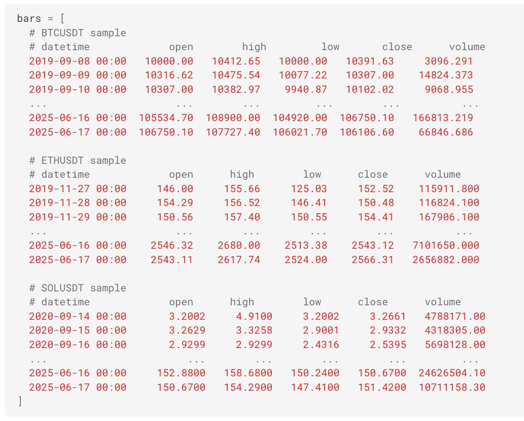
Each DataFrame records daily bars indexed by UTC timestamps.
Rows are truncated for brevity. Note that the data ranges are not equal across instruments, but the algorithm handles dynamic changes in the universe.
We illustrate how the permutation affects marginal distributions. For the period from 2019-09-08 to 2025-06-17, the BTCUSDT series contains 2110 data points. After permuting jointly k=3 times, we plot the marginal price paths using a Japanese candlestick plot.
import numpy as np
import matplotlib.pyplot as plt

k = 3

def plot_japanese_candles(orig, perms):
    fig, ax = plt.subplots(figsize=(15, 6))
    x = np.arange(len(orig))

    for i in x:
        o, h, l, c = orig.iloc[i][['open', 'high', 'low', 'close']]
        ax.vlines(i, l, h, color='black', linewidth=1)
        ax.hlines(o, i - 0.2, i, color='black', linewidth=2)
        ax.hlines(c, i, i + 0.2, color='black', linewidth=2)

    for perm in perms:
        for i in x:
            o, h, l, c = perm.iloc[i][['open', 'high', 'low', 'close']]
            ax.vlines(i, l, h, color='red', linewidth=1)
            ax.hlines(o, i - 0.2, i, color='red', linewidth=2)
            ax.hlines(c, i, i + 0.2, color='red', linewidth=2)

    ax.set_xlabel("Time index")
    ax.set_ylabel("Price")
    ax.grid(True)
    plt.tight_layout()
    plt.show()

perms = [permute_multi_bars(bars) for _ in range(k)]

for i, original in enumerate(bars):
    perm_samples = [perms_j[i] for perms_j in perms]
    plot_japanese_candles(
        original,
        perms=perm_samples
    )
We obtained the following plots:

In red, we show the permuted price paths; in black, the original series.
While the global drift is preserved, all temporal structure has been destroyed in the permuted walks. A cruel but illuminating exercise is to challenge technical analysts to identify so-called ``head-and-shoulders'' patterns on these purely random paths. This is no jibe to discretionary traders - an equally disturbing exercise would reveal that quantitative strategists, armed with modern machine learning tools, commit statistical overfitting — a sin no less severe than the confirmation bias found in technical analysis.
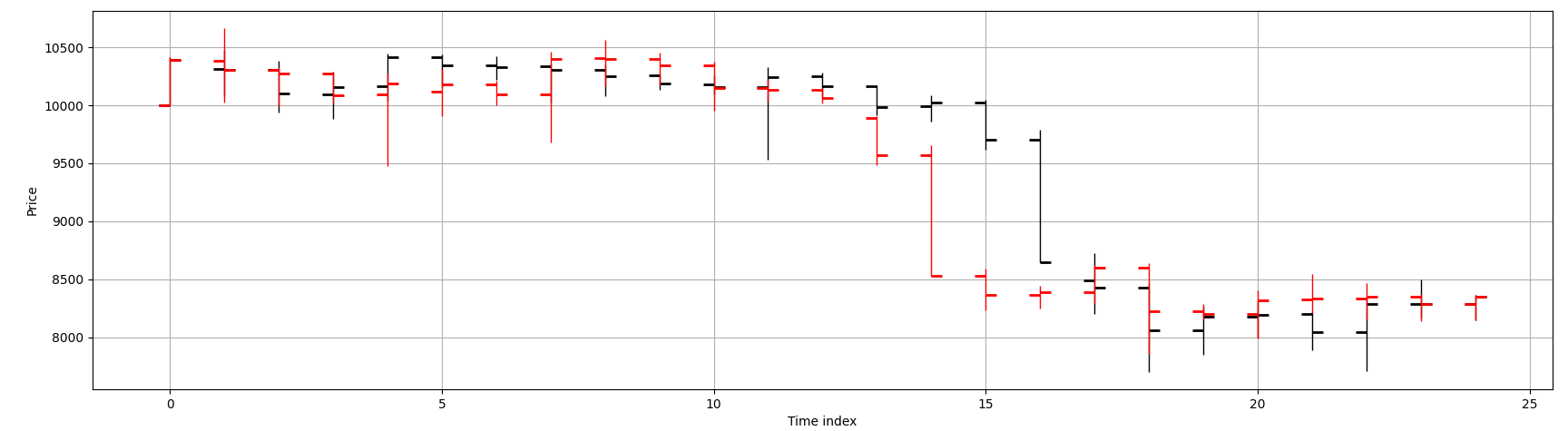
To illustrate the Japanese candlestick representation more clearly, a subsample of 25 consecutive data points is extracted from the BTCUSDT series.
Figure below shows the original price path (black) alongside a single permuted path (red). We should verify that key stylized facts are preserved in our permutations. An example we have taken care to preserve is the distribution of close-to-next-open jumps. Market microstructure effects such as gaps and overnight jumps are not inadvertently distorted. In cryptocurrency futures - this is not particularly interesting since the markets do not close, but would be pertinent in say, equities data.
We also verify that the joint dependence among correlated instruments is preserved. We take the last n=500 overlapping data points and plot their growth paths, each scaled to its initial value. The dotted lines represent the permuted price paths. We observe that the original series are jointly dependent, and so are the permuted series: temporal structure is destroyed both locally and globally, but cross-sectional dependencies remain intact. Consequently, derived models such as static factor models are invariant under the permutation procedure.

The algorithms thus provides a robust foundation for use as a control in scientific experiments investigating machine learning of temporal effects.