
Probabilistic Inferencing for Trading Strategies

Previously, we have discussed classical non-parametric approaches to making probabilistic inferences on attributes of trading strategies based on typical artefacts available.
In this post, we discuss and implement in Python a finite-sample probabilistic bounding method, a unique approach coined Rademacher Anti-Serum by Paleologo, in this new book; The Elements of Quantitative Investing.
We show the RAS implementation on time-series returns from correlated momentum strategies as opposed to uncorrelated random voting machines.
A finite-sample probabilistic bound is a quantitative guarantee on the behavior of a statistic or estimator, for a fixed (finite) sample size, so that for some choice of population quantity theta, statistic theta-hat, epsilon tolerance and delta confidence, we have:
The RAS Method
The RAS method provides a mathematically robust lower bound on the true (out-of-sample) performance of a strategy, given its in-sample performance. RAS “haircuts” your empirical Sharpe to account for multiple testing and model complexity.
In RAS, Sharpe ratio is defined on a per-period basis using standardized returns. If a strategy (portfolio) has weight vector w_{t,n}, and asset return r_t, and covariance matrix Omega_t, then the one-period standardized return is given by;
By standardizing returns each period, we help ensure these performance observations are comparable and (approximately) i.i.d. over time. Using standardized returns as the building blocks means that over T periods, we can treat a strategy’s sequence
as samples from a distribution with mean equal to the true Sharpe ratio. Essentially, instead of computing one Sharpe over the whole sample, we decompose it into T observations of “Sharpe units” for statistical analysis.
The data is then organised into a X[T,N] matrix, where T is the number of time periods and N is the number of strategies, where each entry contains our value of
Each row vector x_t can be assumed to be an an independent draw from some distribution, which asserts no serial correlation. This is roughly true in practice. Each column vector corresponds to a strategy, and strategy-n has some true mean.
The sample mean vector is the empirical performance (the EV of the row-vector in X according to the bootstrap distribution);
RAS framework introduces the Rademacher complexity of the strategies from statistical learning theory to quantify model complexity and potential overfitting. It is defined as follows.
The Rademacher random vector:
where each x_i is drawn from {+1,-1} with equal probability. For instance in a 2-step problem, the Rademacher vectors point to each pole:
Then the empirical Rademacher complexity is defined as
where x^n is the strategy column-n of X. The expectation is taken w.r.t to epsilon.
Since the entries are standardised returns, then
where the approximation holds by LLN, and
since each x_i = +1/-1. So roughly,
the maximum cosine of the angle between the random noise vector and each of our strategy vector. Geometrically, epsilon is a random direction in the T-dimensional space of time-series returns, and the Rademacher complexity tells us how well the set of strategy vectors align with an arbitrary direction. If the strategies are maximally orthogonal, then they span a wide space in T-dim space. Conversely, if strategies are all very similar to each other (highly correlated, spanning a narrow subspace), they cannot align with arbitrary noise directions, and have lower chance of overfitting.
The RAS Bounds
The RAS bounds make a statement like this:
“With high confidence, the real Sharpe/IC of strategy-n is at least its backtested Sharpe/IC minus a complexity penalty (data-snooping haircut) and minus a statistical error term.” The RAS bounds for Sharpe ratio are as such - with probability 1-delta, the true Sharpe satisfies
The last two terms are statistical error penalties that shrink in the number of samples collected, T.
RAS applies a global penalty based on the entire set of strategies, but the lower bound is computed individually per strategy.
RAS thus provides a rigorous decision rule: you might only deploy strategies whose lower-bound Sharpe clears a required threshold to some choice delta.
The RAS Implementation
In practice, we have n-strategies, each of them with a return vector. We can compute standardised returns by normalising against historical vol as a estimate of instantaneous vol.
For implementation, we assume we have some list of dataframes dfs, each with indices of different time ranges. We take maximally overlapping joint periods for the time axis.
To demonstrate complexity penalty depends on orthogonality of the strategies, we choose N=6, and compare between a set of N momentum strategies and N random strategies as follows:
strategies = [
"tszscre_12(close)",
"tszscre_24(close)",
"logret_5(close)",
"logret_20(close)",
"ite(gt(ema_20(close),ema_50(close)),const_1,neg(const_1))",
"ite(gt(ema_50(close),ema_100(close)),const_1,neg(const_1))",
]
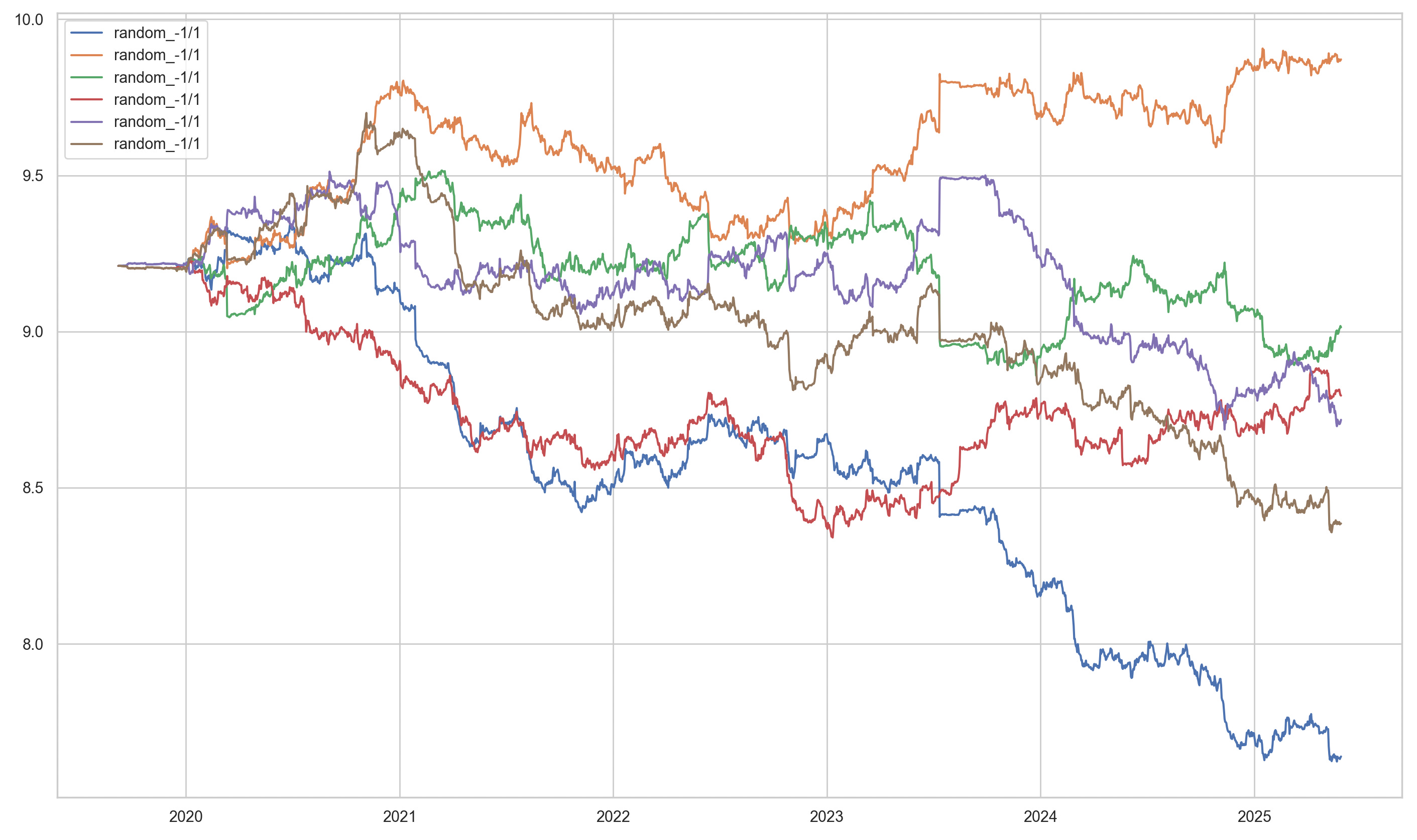
random_strategies = [
"random_-1/1",
"random_-1/1",
"random_-1/1",
"random_-1/1",
"random_-1/1",
"random_-1/1",
]The strategies correspond to trading on the time-series k day z-scores, k logarithmic returns and moving average pairs. The random strategies correspond to random voting machines.
The strategies are tested under the GeneticAlpha engine of the quantpylib library. This engine converts arbitrary signal ranges to valid position sizes using a volatility targeting scheme.
Therefore, although each of the trading strategies have different signal domain, their portfolio sizing and allocations are commensurate due to matching in volatility space. The simulation runs as such:
import pytz
import numpy as np
import pandas as pd
import matplotlib.pyplot as plt
from datetime import datetime

from quantpylib.standards import Period
from quantpylib.datapoller.master import DataPoller
from quantpylib.simulator.gene import GeneticAlpha

keys = {"binance": {}}
datapoller = DataPoller(config_keys=keys)
interval = Period.DAILY

async def main():
    period_start = datetime(2015,10,2, tzinfo=pytz.utc)
    period_end = datetime.now(pytz.utc)
    tickers = [
        "BTCUSDT","ETHUSDT","SOLUSDT",
        "BNBUSDT","XRPUSDT","LTCUSDT","DOGEUSDT"
    ]
    ticker_dfs = await asyncio.gather(
        *[
            datapoller.crypto.get_trade_bars(
            ticker=ticker,
            start=period_start,
            end=period_end,
            granularity=interval,
            granularity_multiplier=1,
            src="binance"
        ) for ticker in tickers]
    )
    dfs = {ticker:df for ticker,df in zip(tickers,ticker_dfs)}

    configs={
        "dfs":dfs,
        "instruments":tickers,
        "granularity": interval,
        "around_the_clock":True,
        "weekend_trading":True,
    }

    for _strategies in [strategies,random_strategies]:

        alphas = [
            GeneticAlpha(genome=strategy,**configs)
            for strategy in _strategies
        ]
        sim_dfs = await asyncio.gather(*[
            alpha.run_simulation() for alpha in alphas
        ])
        r_series = [
            alpha._get_zero_filtered_stats()['capital_ret']
            for alpha in alphas
        ]

        for i,alpha in enumerate(alphas):
            plt.plot(np.log(sim_dfs[i].capital),label=_strategies[i])

        plt.legend()
        plt.show()

if __name__ == "__main__":
    import asyncio
    asyncio.run(main())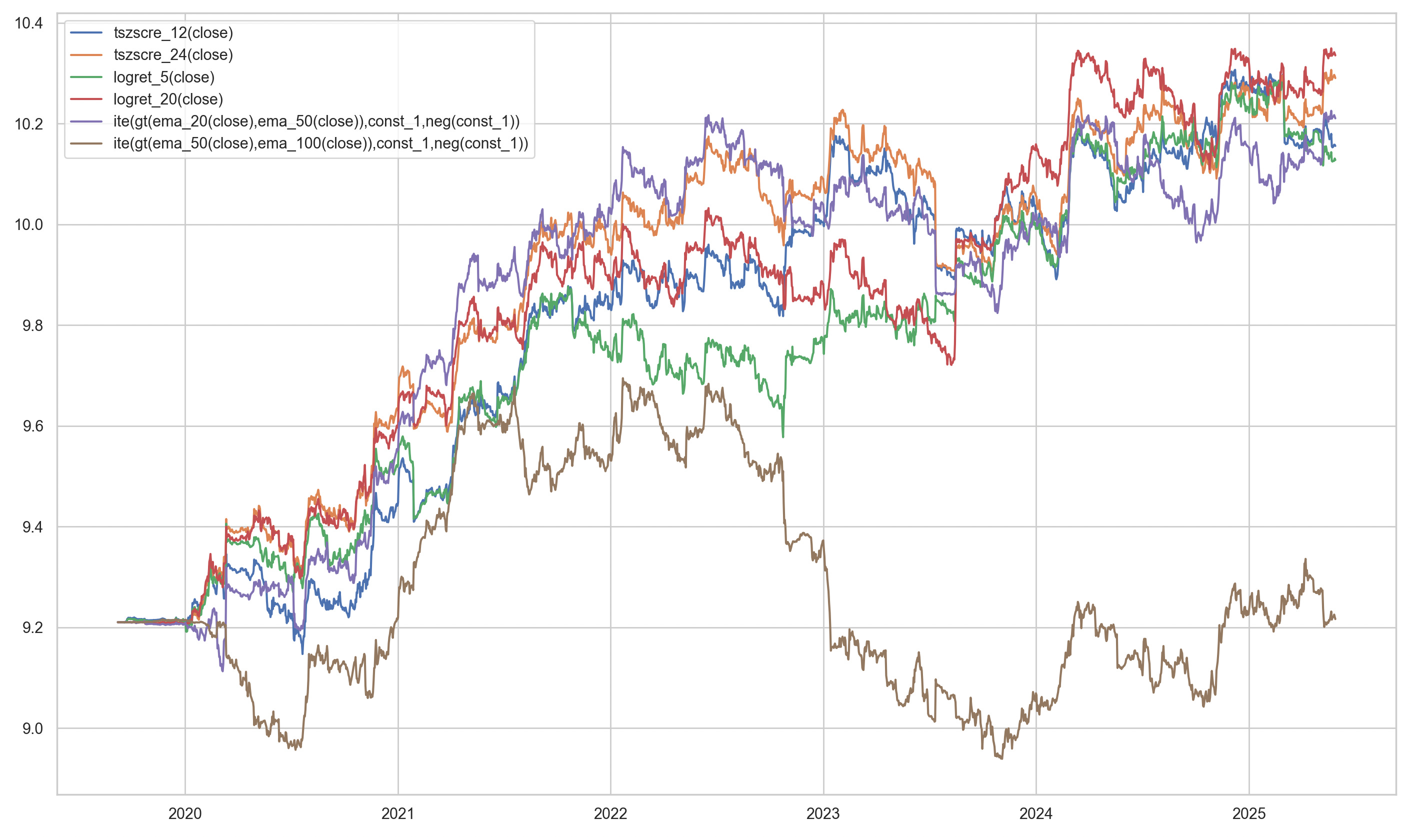
and for random voting machines
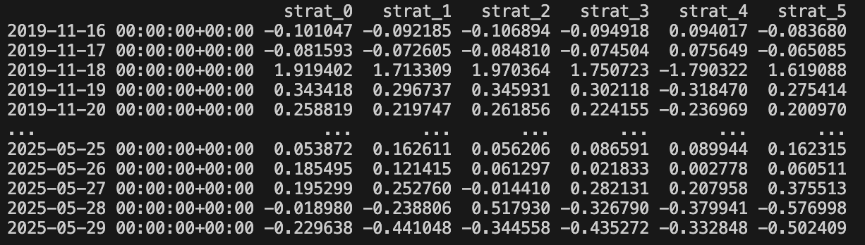
For each of these r_series, we can compute the matrix X:
def construct_matrix_from_series(rets_list, window=20):
    z_scores = []
    for s in rets_list:
        vol = s.rolling(window).std()
        z = s / vol
        z_scores.append(z)

    X = pd.concat(z_scores, axis=1).dropna()
    X.columns = [f'strat_{i}' for i in range(len(rets_list))]
    return X
for something like this:
and estimate the empirical Rademacher complexity:
def estimate_rademacher_complexity(X, n_sim=1000):
    """
    Empirical Rademacher complexity: E[max_n (epsilon^T x_n) / T]
    """
    T, N = X.shape
    X_vals = X.values
    R_vals = []
    for _ in range(n_sim):
        eps = np.random.choice([1, -1], size=T)
        max_proj = np.max(eps @ X_vals) / T
        R_vals.append(max_proj)
    return np.mean(R_vals)
and the RAS bounds are given as such:
def ras_bounds(X, R_hat, delta=0.01):
    T, N = X.shape
    theta_hat = X.mean(axis=0).values

    # Penalty terms
    term_statistical = 3 * np.sqrt(2 * np.log(2 / delta) / T)
    term_multiple = np.sqrt(2 * np.log(2 * N / delta) / T)
    theta_lower = theta_hat - 2 * R_hat - term_stat - term_multiple
    return pd.DataFrame({
        'theta_hat': theta_hat,
        'theta_rademacher': theta_hat - 2 * R_hat,
        'theta_lower_bound': theta_lower,
        'rademacher_penalty': R_hat,
    }, index=X.columns)
and put together;
X = construct_matrix_from_series(r_series, window=20)
R_hat = estimate_rademacher_complexity(X, n_sim=1000)
bounds_df = ras_bounds(X, R_hat, delta=0.05) * np.sqrt(252)
For the momentum group, we obtained the following results
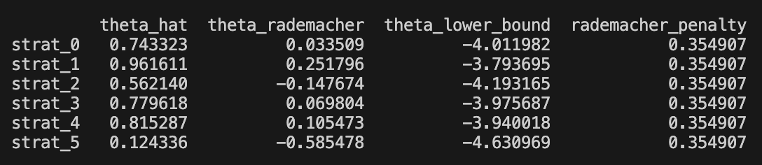
The first column is empirical point estimate of Sharpe, the second column is our (-2*) Rademacher complexity coefficient, and the third column is our finite sample delta-probability bound. The last is the complexity coefficient.
In the random voting machine, we obtained the following
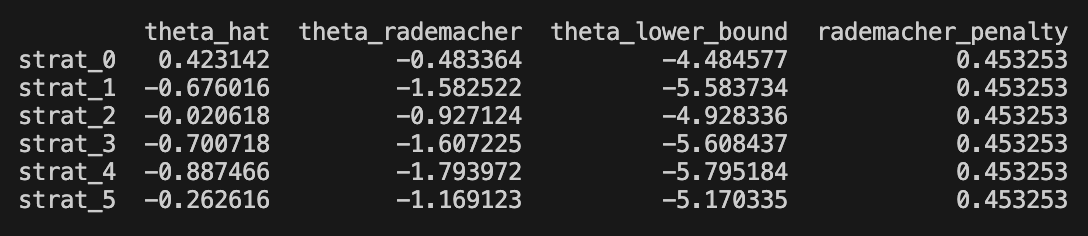
Notably the complexity coefficient is higher due to orthogonality of the random voters. In the book, the strategies for which theta_rademacher > 0 was said to be ‘Rademacher positive’, and strategies with the theta_lower_bound > 0 was said to be ‘positive’ strategies. Notably, none of the strategies are positive, and only the momentum strategies are Rademacher positive.
While not a large sample N or T were employed, the results are coincident of the numerical trials presented on information-coefficient as strategy statistic, and the Rademacher bounds are possibly too conservative. A large part of the conservativeness comes from our lack of data - one may choose to perform this on higher granularities. The bounds are derived on a chain of loose inequalities. In the words quoted from the book:
the path connecting theory and practice is paved with carefully tuned parameters.
_____
Proofs, detailed interpretation and other results are left to the reference text.
All errors are my own.