Quantitative Trading Strategies - How I went from 10k to 100k to 1M (part 4: managing an FX basket)

macroeconomic policy, to statistical modelling and portfolio construction

Hi folks, we previously modelled this before, but there have been significant improvements to the modelling and construction accuracies. We will discuss FX trading today.

Currency desks are commonly divided by geography and market structure: G10, EMFX, LatAm, and so on. In FX, the policy regime plays a significant role in price discovery, and central bank leaning is one of the primary sources of price discovery.

Python Code for replication is provided at the end of the article.

In this series, we will be looking at trading SGD crosses. The MAS manages the Singapore dollar against a basket of currencies through the S$NEER.

The regime is normally described as basket, band and crawl:

• Basket: SGD is managed against the currencies of Singapore’s major trading partners rather than against one bilateral rate.

• Band: the trade-weighted index is allowed to move within an undisclosed policy band.

• Crawl: the slope of that band is reviewed and adjusted as the inflation and growth outlook changes.

These parameters are not disclosed, except for rough “policy guidance”. MAS may intervene through spot or forward FX transactions. Insofar as possible, market forces are otherwise allowed to determine where the currency trades inside the band.

I will leave the economic motivation of these policies as self-reading.

As you may imagine - for a number of business functions (such as fx hedging, speculation) in banks, hedge funds and whatnot - currency desks are undeterred in modelling these parameters.

We will perform such an exercise with public data and construct a trading strategy on a basket of tradable assets. Since MAS explains policy decisions in qualitative language, we will come up with a simple, algorithmic state machine.

In order to assess the quality of our policy recalibration, we will cross-reference with United Overseas Bank (UOB)’s 2019 and 2021 paper.

We will take a look at these subtasks:

• data preparation for statistical modelling

• performing numerical analysis through constrained regression

• algorithmic reconstruction of policy mid, band and width

• portfolio construction from proxy index

• portfolio construction on tradable basket

data preparation for statistical modelling

We require two datasets for the initial statistical model: the official S$NEER history and bilateral SGD exchange rates. Both are available for free from MAS.

The official S$NEER history can be downloaded as an XLSX file from the MAS exchange-rate statistics page. For our purposes the workbook contains two relevant fields:

date          sneer
1999-01-08    100.00
1999-01-15     99.75
1999-01-22    100.10

Each value represents the weekly average S$NEER for the week ending on the stated date. This gives us the dependent variable. We next need a set of explanatory FX rates.

daily FX data

Daily end-of-period exchange rates are available through the MAS API catalogue. The request requires a (free to obtain) API key and returns JSON records. We retain the following currency fields:

USD, CNY, EUR, MYR, JPY, AUD, GBP, IDR,
KRW, THB, CHF, TWD, INR, PHP, VND and CAD

This is our candidate universe, not a claim about the actual basket. The statistical model will determine which currencies receive weight. The raw columns use the following quote convention:

usd_sgd         SGD per 1 USD
eur_sgd         SGD per 1 EUR
jpy_sgd_100     SGD per 100 JPY
idr_sgd_100     SGD per 100 IDR

We normalise this to sgd_xxx convention.

A complete cross-section is available beginning January 2008. The FX data is daily while the official S$NEER series is weekly. Since the target represents a weekly average, we take the arithmetic average of each FX series over the same week.

If W_t is the set of daily observations belonging to week t, the weekly normalized FX level is

\(F_{t,i} = \frac{1}{|W_t|} \sum_{d\in W_t}P_{d,i}.\)

Let S_t denote the official weekly-average S$NEER level for week t. The resulting DataFrame has one row for each common observation week t=0,…,T. We denote this weekly level panel by

\(\mathcal D = \left[ \begin{array}{cccc|c} F_{0,1} & F_{0,2} & \cdots & F_{0,n} & S_0\\ F_{1,1} & F_{1,2} & \cdots & F_{1,n} & S_1\\ \vdots & \vdots & \ddots & \vdots & \vdots\\ F_{T,1} & F_{T,2} & \cdots & F_{T,n} & S_T \end{array} \right] = \left[\mathbf F\mid\mathbf S\right] \in \mathbb R_{+}^{(T+1)\times(n+1)}.\)

The first n columns, F, contain the normalized weekly-average FX levels. The final column, S, contains the corresponding official weekly-average S$NEER levels. In pandas, regression_df is simply the tabular representation of 𝒟.

constructing the basket through restricted least squares

The statistical problem is to infer a dynamic set of currency weights from the weekly level panel 𝒟=[F | S]. We use a weighted geometric basket.

Let S_t denote the official S$NEER level in week t, and let F_t,i denote the normalized weekly-average value of SGD against currency i. We model the changes by differencing the sneer value:

\(\Delta\log S_t = \sum_{i=1}^{n}w_i\Delta\log F_{t,i} +\varepsilon_t.\)

The residual varepsilon_t absorbs anything else not captured by our candidate universe.

Define the weekly S$NEER return

\(s_t=\Delta\log S_t,\)

and the vector of bilateral FX returns obtained from the first n columns of 𝒟,

\(r_t= \begin{bmatrix} \Delta\log F_{t,1} & \Delta\log F_{t,2} & \cdots & \Delta\log F_{t,n} \end{bmatrix}^{\top}.\)

Stacking T observations gives

\(y= \begin{bmatrix} s_1 & s_2 & \cdots & s_T \end{bmatrix}^{\top} \in\mathbb{R}^{T},\)

and

\(R= \begin{bmatrix} r_1^{\top}\\ r_2^{\top}\\ \vdots\\ r_T^{\top} \end{bmatrix} \in\mathbb{R}^{T\times n}.\)

The regression can then be written compactly as

\(y=Rw+\varepsilon.\)

An unconstrained least-squares estimator would solve

\(\widehat w_{OLS} = \arg\min_w \lVert y-Rw\rVert_2^2.\)

This may fit the historical S$NEER well while producing an economically implausible basket. The resulting weights may be negative or may not sum to one.

We know more about the object than ordinary least squares uses. Basket weights should be non-negative, and the complete basket should carry 100% weight. We therefore solve the restricted problem

\(\begin{aligned} \widehat w =\arg\min_w\quad &\lVert y-Rw\rVert_2^2,\\ \text{subject to}\quad &w_i\geq0,\\ &\sum_{i=1}^{n}w_i=1. \end{aligned}\)

The feasible set is the probability simplex

\(\Delta_n = \left\{ w\in\mathbb{R}^{n}: w_i\geq0, \mathbf{1}^{\top}w=1 \right\}.\)

The restrictions give the coefficients an immediate economic interpretation as basket weights.

numerical solution (skip if not interested in the math)

The squared-error objective

\(f(w)=\lVert y-Rw\rVert_2^2\)

is convex, with gradient

\(\nabla f(w) = 2R^{\top}(Rw-y).\)

We solve the constrained problem using projected gradient descent. From a feasible vector w_k, first take an unconstrained gradient step

\(v_{k+1} = w_k-\eta\nabla f(w_k),\)

then project it back onto the simplex:

\(w_{k+1} = \Pi_{\Delta_n}(v_{k+1}).\)

The projection is itself the optimization problem

\(\Pi_{\Delta_n}(v) = \arg\min_{w\in\Delta_n} \frac{1}{2}\lVert w-v\rVert_2^2.\)

Its solution has the form

\(w_i=\max(v_i-\theta,0),\)

where θ is chosen such that

\(\sum_{i=1}^{n}\max(v_i-\theta,0)=1.\)

Intuitively, we subtract a common threshold from the unconstrained vector, set negative coordinates to zero, and choose the threshold so that the remaining weights sum to one.

We use the corresponding step size

\(\eta = \frac{1}{2\lVert R\rVert_2^2},\)

and stop when successive projected weight vectors are sufficiently close:

\(\lVert w_{k+1}-w_k\rVert_2<\epsilon.\)

rolling estimation

We estimate a separate basket for every observation week using the most recent m=260 weekly returns, or approximately five years. This produces a sequence of models rather than one final model, which are the dynamic weights of the basket across time:

\(\widehat w_{t_0}, \widehat w_{t_0+1}, \ldots, \widehat w_T.\)

predicting the S$NEER

A model indexed by week t contains the official S$NEER observation for that week. We shift each fitted weight vector forward by one observation through the preceding observation, ŵ_t-1, and multiply them by the current weekly FX-return vector r_t. The weighted sum is the predicted S$NEER log return. Applying that return to the previous official level gives

\(\widehat S_t = S_{t-1}\exp\left(\widehat w_{t-1}^{\top}r_t\right).\)

How well do the previously estimated basket weights explain the next official weekly move?

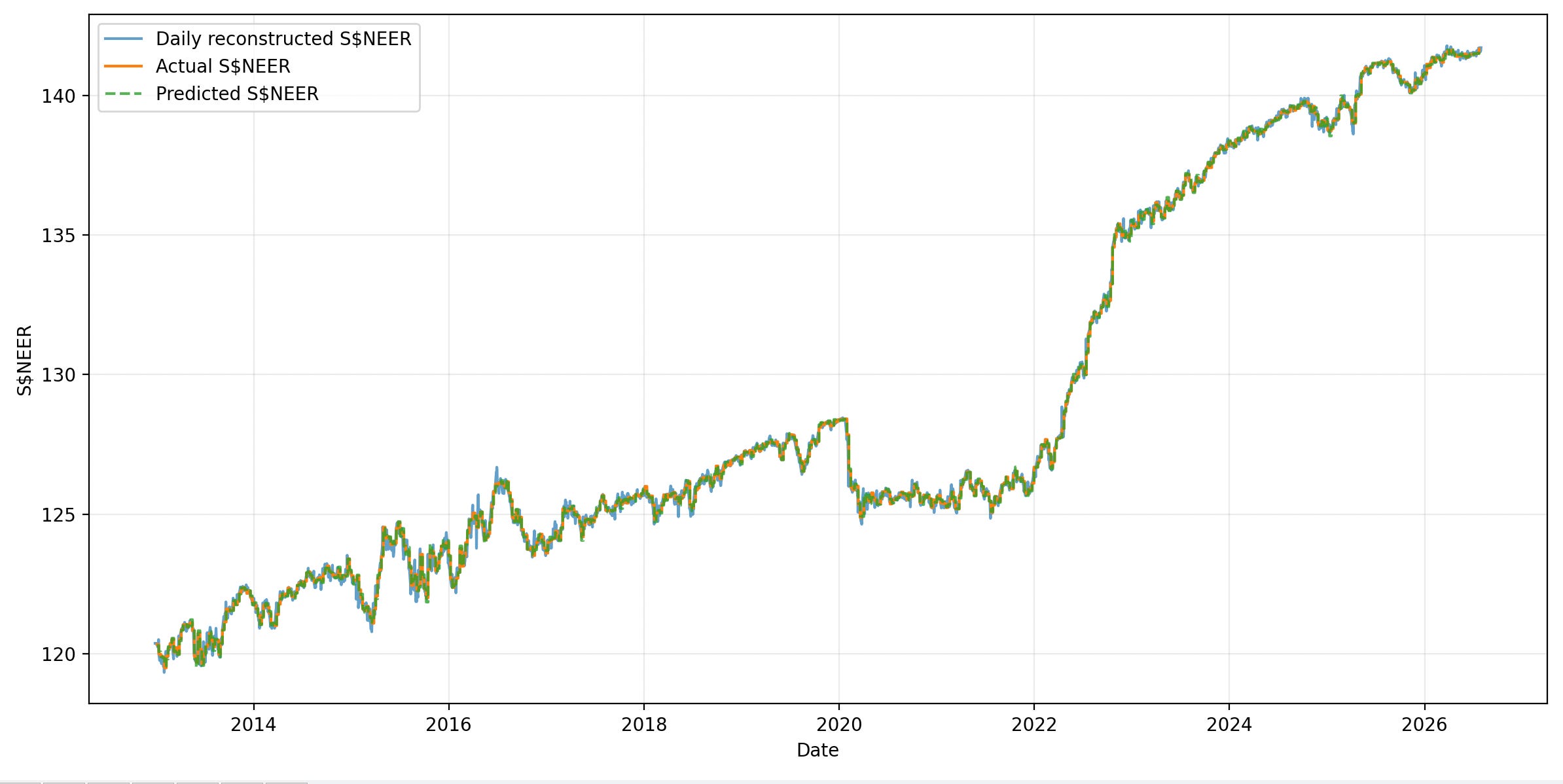
The actual and predicted levels lie almost on top of one another with a 0.972 correlation between the predicted and official weekly log returns, and a 5.07bps in weekly return RMSE.

The fit is strong enough to treat the estimated basket as a useful S$NEER proxy. We have a number of remaining parameters to estimate.

reconstructing the policy band

MAS would make a brilliant X finfluencer, because they are experts in vague-posting. MAS summarises monetary policy statements in roughly this form:

date          slope                 width                   centre
2018-04-13    Increase slightly     -                       -
2020-03-30    Set at 0%             -                       Re-centre downwards
2022-04-14    Increase slightly     -                       Re-centre upwards

Our job is to translate qualitative policy language into a deterministic state machine.

Let g denote the annualized slope of the midpoint and let h denote the log half-width of the band. An unchanged field carries its previous value forward. Every other phrase updates one component of the policy state:

• increase very slightly: g ← g+0.5δ

• increase slightly: g ← g+δ

• increase: g ← g+2δ

• reduce slightly: g ← max(0,g-δ)

• reduce: g ← max(0,g-2δ)

• set at 0%: g ← 0

• widen slightly: h ← 1.25h

• widen: h ← 1.5h

• restore narrower band: h ← h₀

• re-centre: reset the midpoint to the prevailing (predicted) S̃_d

The rules are symmetric. The zero floor prevents a sequence of reductions from implying a negative slope due to MAS slope policy since the outset.

We set one slope tick to δ=0.5% per annum, use a baseline log half-width of h₀=0.02, or approximately 2% on either side of the midpoint, and anchor the April initial slope at 2% per annum.

This is aligned with the UOB’s paper. Once these values are fixed, the same rules are applied across the entire time series; there is no additional parameter fitting.

evolving the midpoint

Let M_d be the policy midpoint on day d. Between re-centring decisions, its log level accumulates the prevailing annualized slope:

\(\log M_d = \log M_{d-1} + g_{d-1}\Delta\tau_d,\)

where Δτ_d is the fraction of a year elapsed since the preceding observation. On a re-centring date, we reset M_d to the prevailing reconstructed S$NEER and continue accumulating drift from the new base.

The upper and lower boundaries are then

\(L_d=M_d\exp(-h_d), \qquad U_d=M_d\exp(h_d).\)

Using a geometric band keeps both boundaries positive and makes widening symmetric in log-return space.

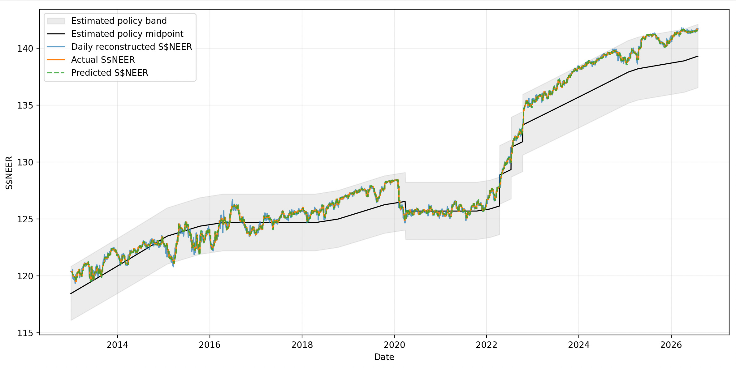
We have now constructed a parsimonious model calibrated against a deterministic state machine, and verified that results are somewhat in line with a reputable bank. If we are economist, we would be happy, but as traders, we make no money from this…

But how may we construct a continuous portfolio from this?

portfolio construction