

PSA: we have an ongoing, 1-week 50% discount on all subs.

A factor model is motivated by the observation that market movements are primarily driven by a relatively small number of common sources of risk. Assets may have thousands of individual return streams, but much of their variation is shared: broad market movements, industries, economic characteristics, liquidity conditions, or latent statistical relationships. The purpose of a factor model is to separate these common movements from asset-specific noise.
There are three broad approaches: Fama-style (time-series) portfolio factors, statistical factor models such as PCA, and Barra-style (cross-sectional) exposure models. They differ not merely in interpretation, but in the direction of estimation, the information supplied to the model, and the quantity being estimated.
Getting timely exposure to desirable factors — and hedging undesirable ones — is a primary concern of smart-beta funds and are a TRILLION dollar industry.
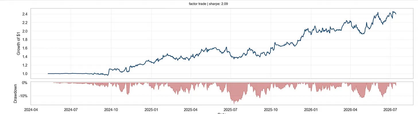
Factor analysis in crypto is still nascent. This article focuses on Barra-style models and how I actively trade them to enhance my pnl.
The full implementation is included at the bottom.
We will touch lightly on the first two, and then detail a Barra-style analysis with code.
Fama-style
A Fama-style factor is defined as the return of a portfolio. For example, a simplified value factor might be
More generally, if (pk,t) contains the asset weights of factor portfolio (k), then
Once these factor-return histories have been constructed, the exposure of an individual asset is estimated through time:
The factor-return matrix (F) is known. The regression estimates (βi):
For a single, demeaned factor,
Fama-style models are motivated by economic hypotheses about expected returns. Is a manager’s apparent alpha simply compensation for exposure to known factor strategies? Is our portfolio (statistically) significantly just some beta against a factor portfolio?
For a portfolio with estimated factor betas (βp),
Statistical-style
A statistical factor model begins with the complete return matrix:
where rows are dates and columns are assets. It seeks a lower-dimensional approximation:
where F ∈ ℝT×K contains the statistical factor returns and L ∈ ℝN×K contains the asset loadings. In principal components analysis, first estimate the asset covariance matrix:
of demeaned returns. Decompose it as
The first (K) eigenvectors define the principal directions:
and the corresponding factor scores are
The resulting rank-(K) reconstruction is
Unlike the Fama regression, however, neither the factors nor the loadings are specified economically.
These are motivated mainly by dimensionality reduction. If hundreds of assets share a few dominant covariance patterns, the researcher may want to discover those patterns without imposing characteristic taxonomy.
Barra-style
The focus of our post, is the Barra-style model. We will first discover it’s mathematical basis, and then use them to identify sector performance.
We begin by specifying each asset’s exposures. On date (t),
contains exposures to K factors, such as categories, industries, countries, or continuous styles such as size and momentum.
The model then examines the cross-section of asset returns on that date:
The exposures (Bt) are known. The factor returns (ft) are estimated using the (N) assets observed on that date.
This regression is repeated for every date, therefore produces a time series of factor returns from a sequence of cross-sectional regressions.
Barra-style models are motivated by the need to describe the current economic composition of a portfolio. Rather than waiting for a long return history to reveal a portfolio’s betas, the manager declares or measures the underlying asset exposures directly.
Repeating the cross-sectional regression each day produces a synthetic return series for every factor. By extension, if sector inclusion is defined as a factor, we obtain the synthetic return of the sector performance.
They are useful to:
portfolio managers performing return attribution;
risk managers estimating common and specific risk;
traders neutralising unwanted industry or style bets;
isolating sector performance for smart beta plays.
The factor return has a different meaning from a Fama-style factor. It is the return attributed to one unit of exposure after controlling for the other exposures in the cross-sectional regression.
Example'; crypto Barra model
We will demonstrate the categorical Barra analysis here using a reduced four-asset problem with two categories. The full regression code can be found at the bottom.
Let’s begin.
Suppose our universe contains four assets:
BTC — L1; daily return 4%; liquidity score 4.
ETH — L1; daily return 2%; liquidity score 2.
DOGE — Meme; daily return 8%; liquidity score 1.
PEPE — Meme; daily return 6%; liquidity score 1.
The objective is to estimate three returns:
The market factor represents the weighted return of the crypto universe. The category factors represent L1 and Meme performance relative to that market.
1. Construct the return vector
For each asset, the daily close-to-close return is
Collect the four asset returns into the vector
This is the dependent variable in the daily cross-sectional regression.
2. Construct the regression weights
For each day, determine asset’s regression weight. Reasonably, we may choose the square root of its preceding 30-day dollar volume:
The weights are then normalised:
Our simplified liquidity scores are
Since they sum to eight, the normalised weights are
The WLS weighting matrix is simply diag(w).
BTC contributes half of the regression weight, ETH contributes one quarter, and DOGE and PEPE each contribute one eighth.
3. Construct the exposure matrix
Every asset has market exposure equal to one. It also has exposure equal to one to its assigned category.
The exposure matrix is
for columns [market, L1, Meme] and rows [BTC, ETH, DOGE, PEPE].
Each day, the regression equation is given by (solve for f)
For instance,
The model assigns the same fitted common return to assets in the same category. Differences between the individual asset returns in a fitted category return remain in the residuals.
4. Remove collinearity problem
The market column is equal to the sum of the two category columns:
Consequently, the exposure matrix does not have full column rank.
For a particular solution
and any constant a,
produces exactly the same fitted asset returns.
We may solve this by requiring the liquidity-weighted average category return to equal zero.
5. Reduction of Degree of Freedom
Let the aggregate weight of category c be
In our example,
We impose
Substituting the category weights,
The constraint vector is therefore
and the constraint is
The leading zero means that the market coefficient is not directly constrained.
6. Solving the constrained WLS
We minimise the weighted squared residuals:
subject to
Introduce a Lagrange multiplier λ:
The first-order condition with respect to f is
Rearranging,
The first-order condition with respect to λ is
Combining the two equations produces the KKT system:
For our example,
The weighted return vector is
The first element is the weighted return contribution of the whole market:
The second is the weighted contribution from L1 assets:
The third is the weighted contribution from Meme assets:
The complete system is
Solving gives
The constraint is satisfied:
7. Interpretations
The weighted return of the L1 category is
The weighted return of the Meme category is
The category coefficients are the differences between these category returns and the weighted market return:
The fitted common return for an L1 asset is
The regression therefore tells us:
the weighted market returned 4.25%;
L1 underperformed the market by 0.9167%;
And the same exercise applies to the Memes category.
The residuals describe the returns not explained by category membership.
For BTC,
8. Repeat the analysis through time
The same cross-sectional regression is repeated for every date t. Each regression produces one market return and one relative return for every represented category:
Stacking the daily estimates produces a synthetic return history for every category/sector.
For example,
is the estimated history of the crypto meme-sector relative to the weighted crypto market. If we take these as ‘sector returns’ and compound them from 1, we essentially have a synthetic sector index. This is (theoretically) tradable with a factor-mimicking portfolio.
9. Recover the factor-mimicking weights
The estimated coefficients are linear combinations of the asset returns. We may therefore recover asset weights that reproduce them exactly.
For the market factor, the mimicking weights are the normalised regression weights:
For category c, the mimicking weights are
For L1, this gives
These weights sum to zero:
Their realised return is
For Meme,
Its return is
This exactly reproduces the L1 factor return.
The category factor can therefore be interpreted as a long position in the weighted category basket and a short position in the weighted market basket.
The factor-mimicking portfolio exists exactly in the mathematics. Essentially, what we have done is to transform quantitative analysis from price space to factor space, using statistical categorical analysis. In the process, we might
better appreciate crypto asset returns as a mixture of factors/sectors
construct a more informed portfolio by reducing noise in our samples
For instance, using “theoretical” factor-mimicking portfolios, we may look to construct a long-short delta neutral portfolio for “bullish sectors” against “bearish sectors”. Or we may look to “enhance” our trend construction from the previous post to trading in the factor space, subject to same considerations of portfolio construction that were discussed.
Code:
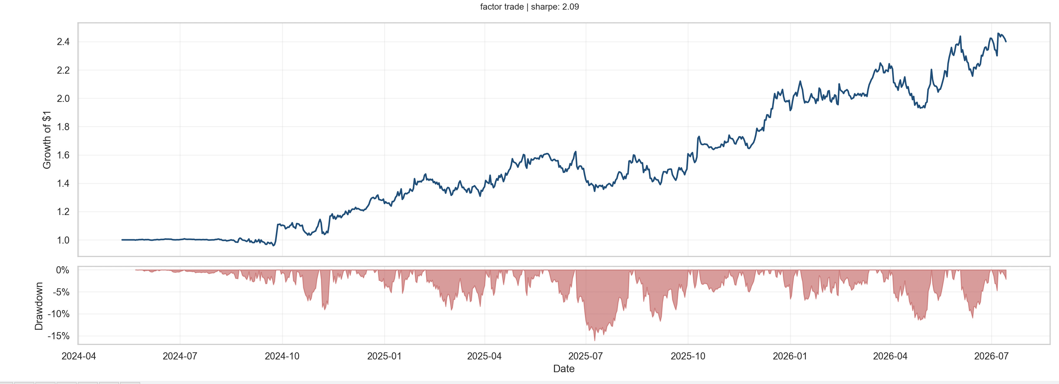
Let’s take a look an example construction of the above test to a universe of hundred tickers from Binance and Python code.