Quantitative Trading Strategies - How I went from 10k to 100k to 1M (part 1: trend my friend)

trend following over the years, with code

PSA: we have an ongoing, 1-week 50% discount on all subs.

Quantitative Trading Strategies - How I went from 10k to 100k to 1M (new series intro)

IN my first quant internship, I was tasked with testing commodity futures skew effects.

pm: "how did you account for contract roll"

me: "treated them as continuous, sometimes it's contango sometimes backwardated, so. it's small approximation error"

pm: 😑

In trading, a lot of effects and strategies are known. Index rebalancing, stat arb, yield curve arbitrage, market making - are all known strategies. The devil is in the details, and like my old self, doing something and doing something right are completely different things. If you are targeting these strategies, fantastic! You are in the right arena. For those testing some inverse shoulder rsi combo schtick, it’s time to come around. No shame in where the journey starts.

This article is dedicated a little bit to that - when asked about how one should “start their quant journey”, I always default to this one - a fantastically simple strategy that opens up a ton of critical questions that expand to more complex strategies. For example

• Execution fees and optimal rebalancing

• Signal quantisation

• Volatility and square root laws

• Diversification

• Backtesting sanitation

• Signal transformation

• Risk targeting/management

• Order automation

It is also one of the strategies that is “slow enough” that can be handled manually, and where different components mentioned above can be automated “one-at-a-time”, which is the good old principle of abstraction and core principle of building complex systems.

Our next post will continue on factor trading and how I leverage ‘smart-beta’ strategies to enhance portfolio returns.

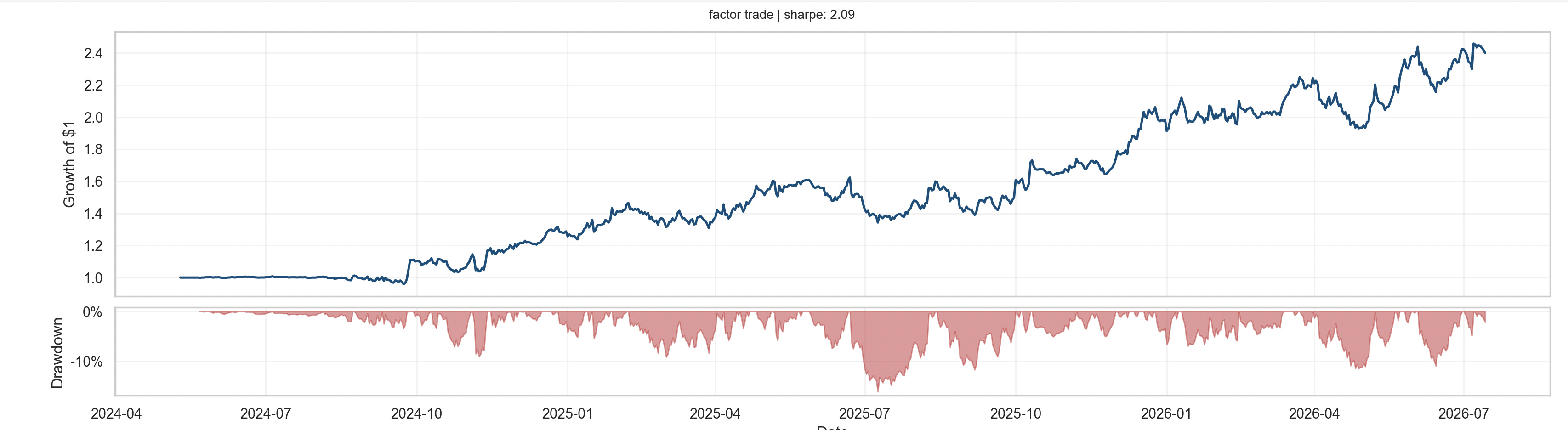
Shall we begin?

(Code is attached at the bottom.)

Signal is the easy part.

The high-level rule is simple: buy markets that are going up and sell markets that are going down. It gives us a strategy whose intuition can be stated in one sentence, and then there is everything else.

\(\text{market data} \rightarrow \text{trend signal} \rightarrow \text{forecast} \rightarrow \text{position} \rightarrow \text{portfolio} \)

Until we specify how strongly to trade the signal, how much risk to allocate to each asset, how contracts are sized, when trades are executed and how costs are charged, it’s not a quantifiable test.

Trend following is therefore a useful first quantitative strategy for two reasons. It is simple enough that we can intuit the entire research process, while being rich enough to expose common lapses in framework and backtesting.

Moskowitz, Ooi and Pedersen document this effect across equity-index, currency, commodity and bond futures. A diversified portfolio of these signals produced returns with little exposure to conventional asset-pricing factors and tended to perform well during large market moves.

Let’s just say, there is a ton (two centuries) of evidence supporting trend following: A Century of Evidence on Trend-Following Investing and Two Centuries of Trend Following.

As they say, if it’s robust, simple does the trick. The simplest discrete signal is the sign of a trailing return:

\(s_{i,t} = \operatorname{sign} \left( \frac{P_{i,t}}{P_{i,t-h}}-1 \right)\)

The forecast is +1 when the asset has appreciated over the previous h periods and -1 when it has depreciated.

A moving-average crossover produces a similar binary rule:

\(s_{i,t} = \operatorname{sign} \left( MA^{\text{fast}}_{i,t} - MA^{\text{slow}}_{i,t} \right)\)

Now imagine if you were thirsty, and you could only drink or not drink a litre at a time. That would be miserable. A continuous forecast tries to retain information about trend strength.

A continuous forecast distinguishes between a weak and strong trend. It can also move gradually through zero rather than jumping directly from fully short to fully long. Continuous rules based on the statistical strength of a trend can materially reduce turnover without a statistically significant performance penalty.

One possible construction is a volatility-normalised trailing return:

\(f_{i,t} = \operatorname{clip} \left( \frac{\sum_{k=1}^{h} r_{i,t-k}} {\hat{\sigma}_{i,t}\sqrt{h}}, -f_{\max}, f_{\max} \right)\)

In more nuance, weak trends appear to persist, but the relationship eventually saturates. We know this from the Potters and Bouchaud paper. The appropriate forecast may therefore look less like an infinitely increasing linear function and more like a clipped or saturating one. A sensible forecast transformation is often saturating:

\(\tilde f_{i,t} = \tanh\left(\frac{f_{i,t}}{c}\right)\)

Can I Have One HubbaHubba of Egg Contracts? On Risk.

Said no-one ever.

Suppose Bitcoin and interest-rate futures both produce a forecast of +1. What does this even mean? Giving them the same dollar exposure makes no sense from an economic standpoint. A standard normalisation feature to encode a dimensionless forecast is the forecast annualised return volatility of asset i:

\(u_{i,t} = b_i \frac{f_{i,t}}{\hat{\sigma}_{i,t}}\)

where b_i is an instrument or asset-class risk budget.

The inverse-volatility term gives smaller positions to volatile assets and larger positions to quiet assets. With binary forecasts and equal risk budgets, each instrument contributes approximately the same standalone volatility before correlations are considered.

Extending this framework, asset normalisation does not guarantee portfolio risk stability. 10 contracts long A and 10 contracts short B is a different portfolio from 10 contracts long in each. Instruments are correlated, correlations are dynamic, and the positions are too.

Let u_t be the vector of preliminary exposures and let Sigma be the forecast covariance matrix of asset returns. The forecast volatility of the preliminary portfolio is:

\(\hat{\sigma}_{p,t} = \sqrt{u_t^\top \hat{\Sigma}_t u_t}\)

Given a portfolio volatility target, the final exposure vector is

\(w_t = \frac{\sigma^\text{target}} {\hat{\sigma}_{p,t}} u_t\)

scaling the whole portfolio so that its forecast volatility equals the target.

There are therefore two distinct pieces of risk management:

1. Asset-level normalisation prevents volatile instruments from dominating the portfolio performance.

2. Portfolio-level scaling adjusts total leverage based on dynamic correlations and the realised volatility of the combined strategy in relation to target.

Volatility targeting has a wider literature of its own. Reducing exposure during high-volatility periods improves the historical Sharpe ratios of several risk factors.

We Live in the Real World

For a linear contract, a simplified conversion from notional weight to units is

\(q_{i,t} = \frac{A_t w_{i,t}} {P_{i,t}M_iX_{i,t}}\)

where A is the portfolio capital, P is the contract price, M is contract multiplier and X is the currency conversion. The position must then respect integer contract quantities, minimum order sizes, tick sizes, leverage limits and venue-specific margin rules. This may surprise some crypto traders, but you can’t always buy 0.0001 of $MONKEY coin in liquid futures markets where standardised contracts trade in (large) fixed sizes. Accordingly, this tracking error can play a part in ‘which universe of assets’ are sensibly tradable for hedge funds - even when AUM is minimally tens of millions! When generating backtests, we need to be careful about directionally correct and economically meaningless results.

\(r_{p,t+1} = w_t^\top r_{t+1} - C(\Delta w_t) - \operatorname{Carry}_{t+1}\)

Next on the chopping board of reality are fees. The cost function includes commissions, bid-ask spreads, slippage, market impact and carry/funding costs.

Thankfully, when doing longer-term trend following, fees are more…secondary class citizens. However, as you evolve in your career as a trader, or look at higher frequency trading, you, too, will come to obsess about fees. But for now, in this post, we can be abit more cavalier about it.

To be frank, cost management and proper backtesting principles probably deserve an entire series on its own, but that borders on the HOW rather than the WHAT, and I promised not to bore you with the how in this series. I do have an entire post on statistical inferencing for backtest validation, if you are interested.

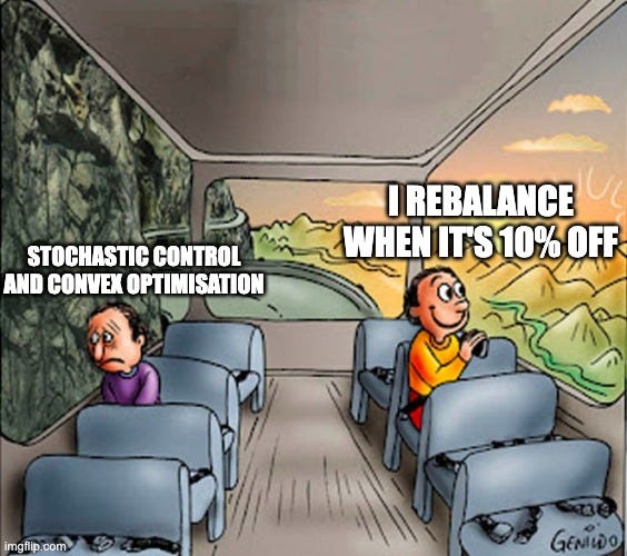
So, for now - COST IS IMPORTANT, and non-negligible, and ideas from optimal control theory suggest that we should…have continuous signals but not continuous positions. This prevents us from “flip-flopping” our holdings and paying the broker or the market maker excessively. Fortunately, we can get 95% of the way there with 5% of the brain: by applying “positional inertia” - the inertia to trade into target position when the current position is sufficiently close to the target.

The “rough-ideal” for inertia levels can be set by setting average trading costs and varying inertia levels, and then simply doing a walk forward backtest to find the optimal tradeoff. If robustness is anywhere found, a reasonable band will appear. Generally, the more noise (or low Sharpe your cost-free strategy is), the larger should be your inertia threshold. If your signal is all-noise, then you should just sit on your hands and stop trading all together.

Code

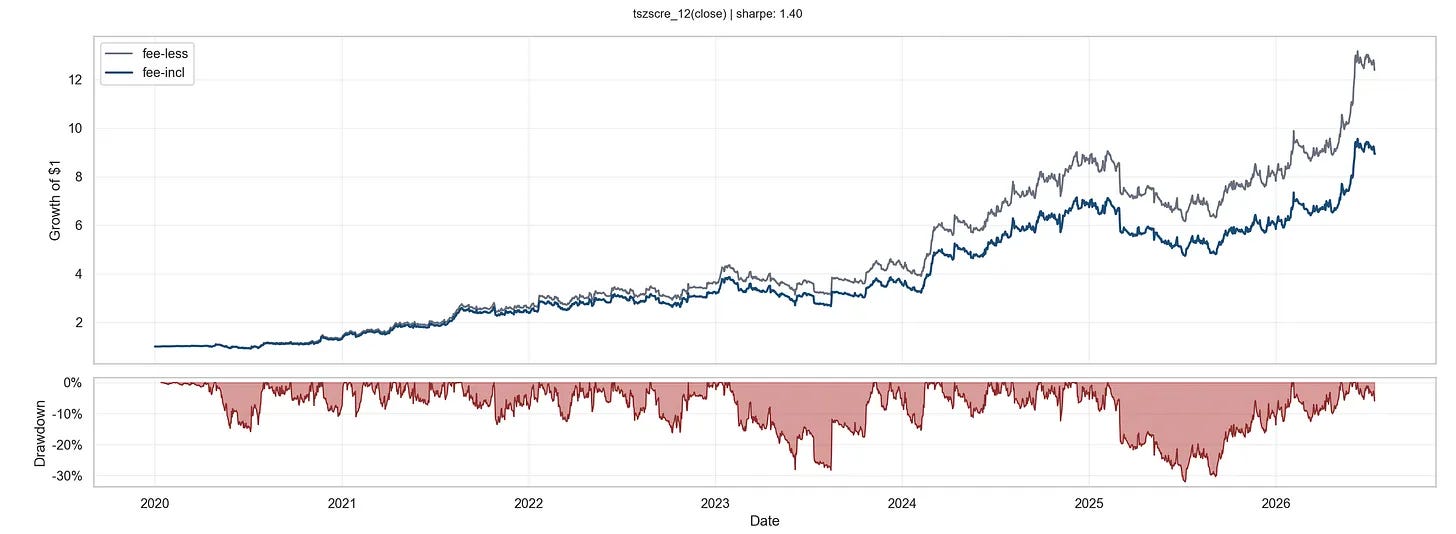
Comparing with and without costs:

From a code perspective, it is critical from a research infrastructural standpoint to encompass all (or most) of the above concerns in a parsimonious framework. What separates novice traders from more sophisticated quantitative analysts is the research harness.