HFT MM: Detailed Guide to Queue Modelling and Calibration

Note that terminal access pass cost increases in 3 days.

Queue Modelling in HFT Simulations

In HFT market making, running high-fidelity tick-data simulations is particularly challenging. It is easy to invent false artefacts around market microstructure which generate positive PnL but do not hold in practice. This is because we make assumptions around important considerations like latency, queue priority, market impact and so on.

At a high level, an execution simulation has to be concerned with:

1. When our order lands on the order book.

2. When our cancellation lands on the order book.

3. Our estimated queue position relative to exogenous market actions.

4. The impact of other traders reacting to our orders.

5. The endogenous impact of our orders on the simulated order book.

The first two are latency problems. Order-latency distributions may be backed out from our own order traces, with an appropriate sampling method. Similarly, an order remains live while its cancellation is in flight. Market events between these timestamps have to be applied against the correct exchange-side state.

The third is the usual queue-position problem: how much liquidity is ahead of us, and how does that quantity change as trades, submissions, modifications and cancellations occur?

The fourth is a much harder problem. Historical replay tells us how other participants behaved in the observed market. It does not tell us how they would have behaved had our simulated order been larger, smaller or absent. Modelling this properly requires an endogenous model of external order flow - we will leave that outside the scope of this post.

Our focus in this post is the theoretical basis of points 3 and 5. In particular, we will separate two ideas which are often mixed together under “queue modelling”:

• Impact modelling: how should our order change the displayed and matchable liquidity inside the replay?

• Position modelling: where should our order sit, and how should exogenous events change the quantity ahead of it?

Given different choices to queue models, we also want to know how we may tune or calibrate them from a statistical framework.

MBO vs MBP

When we have market-by-order data—MBO (L3)—queue reconstruction is relatively straightforward. The feed identifies individual order submissions, modifications and cancellations. Assuming price-time priority, we can reconstruct the orders at a level and insert our own order according to its exchange-arrival timestamp.

When an external order is cancelled, we know which order left the queue. We therefore know whether the cancellation occurred ahead of or behind us.

In crypto, we typically have market-by-price data—MBP (L2). The feed gives us aggregate quantity at each price but does not identify the orders making up that quantity.

Consider a level displaying ten units. The level later falls to six. We know that four units have left, but the L2 update does not tell us where those units were in the queue.

If they were ahead of our order, our position has improved by four. If they were behind us, our position has not improved at all. This is the crux of estimating queue priority and building queue models.

An optimistic model may remove it from ahead of us; a pessimistic model may remove it from behind us; a probabilistic model sits somewhere between the two.

Before we get to this position problem, there is a lesser asked but equally important question.

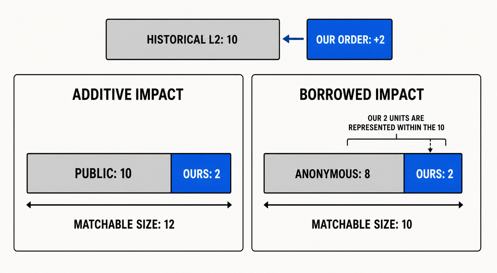
Suppose the historical L2 book displays ten units at a price and we submit a two-unit order. Should the simulated book now display twelve units, or should our two units be treated as part of the ten already observed?

There is no one-size-fits-all answer. It depends on our order size, the liquidity of the market and, importantly, whether we were already quoting on the book used to record the historical data. This is an orthogonal question to point 4—should our orders should be represented inside the public book?

The good news is that we can answer such difficult questions by tuning our queue models and parameters and comparing them against empirical results, thereby reducing the dimensions of our problem.

In QuantPylib, the L2 and L3 order books are mapped through a common data structure. QuantPylib’s replay logic implements the discussed policies.

We will discuss how synthetic L2 MBP data can be projected onto an L3 MBO book by separating liquidity into anonymous and private sizes, over which we may configure different queueing and impact policies.

Projecting L2 into an L3 State

Consider a single price level displaying ten units of liquidity. Our two-unit order lands at the same price.

There are two ways to project the new state.

Additive Impact

The additive model is simple. Historical public liquidity and our private liquidity are disjoint.

If the observed L2 quantity is L and our total private quantity is O, the matchable size is:

\(T=L+O\)

Our order is appended to the price level when it arrives. Subsequent L2 updates change the public quantity independently of our order. Cancelling our order removes its entire remaining size.

Borrowed Impact

The borrowed model is more challenging because public and private liquidity are no longer disjoint accounting buckets.

For one side and price, define:

• L: public size reported by the historical L2 feed;

• O: total size of our active private orders;

• B: private size borrowed from—and therefore already counted in—the historical public size;

• E: anonymous external liquidity represented in the synthetic L3 book;

• T: total physical quantity available to the matcher.

The following invariants must hold:

\(E=L-B\)

\(T=E+O=L+O-B\)

\(0\leq B\leq\min(L,O)\)

For a fully borrowed-impact model, we target:

\(B=\min(L,O)\)

and therefore:

\(T=\max(L,O)\)

Probably confusing, so let’s walk through some interesting cases.

Private size exceeds the observed level

Suppose the historical level displays three units and we submit an order for five:

\(L=3,\qquad O=5\)

The private order can borrow only the three units available in the public observation:

\(B=3,\qquad E=0,\qquad T=5\)

All three public units are represented by our order. The remaining two units are necessarily additive.

The cancellation behaviour is slightly less obvious. If we cancel the five-unit order, only its two additive units should disappear from the physical book. The three borrowed units still belong to the historical public observation and must return as anonymous liquidity:

before cancellation:
[ours: 5]

L = 3, O = 5, B = 3, E = 0, T = 5

after cancellation:
[anonymous: 3]

L = 3, O = 0, B = 0, E = 3, T = 3

Cancelling the private claim does not cancel the historical market.

Public size moves through private size

Now suppose our private order has size ten while the historical L2 level displays five:

L = 5, O = 10, B = 5, E = 0, T = 10

The public level then rises from five to eight:

L = 8, O = 10, B = 8, E = 0, T = 10

The physical matchable size does not change. Three more units of our private order simply become borrowed from the updated public observation.

If the L2 level subsequently rises to twelve:

L = 12, O = 10, B = 10, E = 2, T = 12

Our full ten-unit order is now borrowed, while the remaining two public units must be represented as anonymous liquidity that queues behind our owned orders.

The reverse case - suppose the public level falls from twelve to seven:

before:
L = 12, O = 10, B = 10, E = 2, T = 12

after:
L = 7, O = 10, B = 7, E = 0, T = 10

The private order remains physically matchable for ten units. The two anonymous units disappear, while three units of the private order lose their borrowed attribution and become additive.

The different impact models fundamentally discuss the philosophy of whether our simulated orders should be treated as additional liquidity, or as liquidity already represented in the observed market data.

Queue Position Policies

Once the impact policy has produced a synthetic L3 level, the queue policy determines how exogenous reductions change our position.

New public liquidity joins the tail. Historical trades consume liquidity from the head. The ambiguous event is an L2 size reduction: did the disappearing liquidity sit ahead of us or behind us?

Optimistic and pessimistic bounds

Consider a borrowed-impact book with ten public units. We submit an order for two:

[anonymous: 8] [ours: 2]

The public level then rises from ten to fifteen. The new liquidity joins the tail:

[anonymous: 8] [ours: 2] [anonymous: 5]

The level subsequently falls back to ten.

An optimistic, front-cancellation policy removes the five units from the head:

[anonymous: 3] [ours: 2] [anonymous: 5]

Our queue position has improved by five. A subsequent trade for five units consumes the three anonymous units ahead of us and fills our two-unit order.

A pessimistic, back-cancellation policy removes the five units from the tail:

[anonymous: 8] [ours: 2]

Our position has not improved. The same five-unit trade does not reach us.

The market data is identical in both cases. Only the queue policy changes.

Probabilistic queue models

The optimistic and pessimistic models are useful bounds. A probabilistic model allocates the reduction between liquidity ahead of and behind our order.

Let:

• A: anonymous quantity ahead of our order;

• H: anonymous quantity behind our order;

• C: observed L2 reduction.

Define the relative queue position:

\(x=\frac{A}{A+H}\)

A simple probability function is:

\(p_{\text{ahead}}(x) = \frac{f(x)} {f(x)+f(1-x)}\)

where:

\(f(x)=x^\gamma\)

The exponent γ > 0 controls the curvature of the cancellation-probability function.

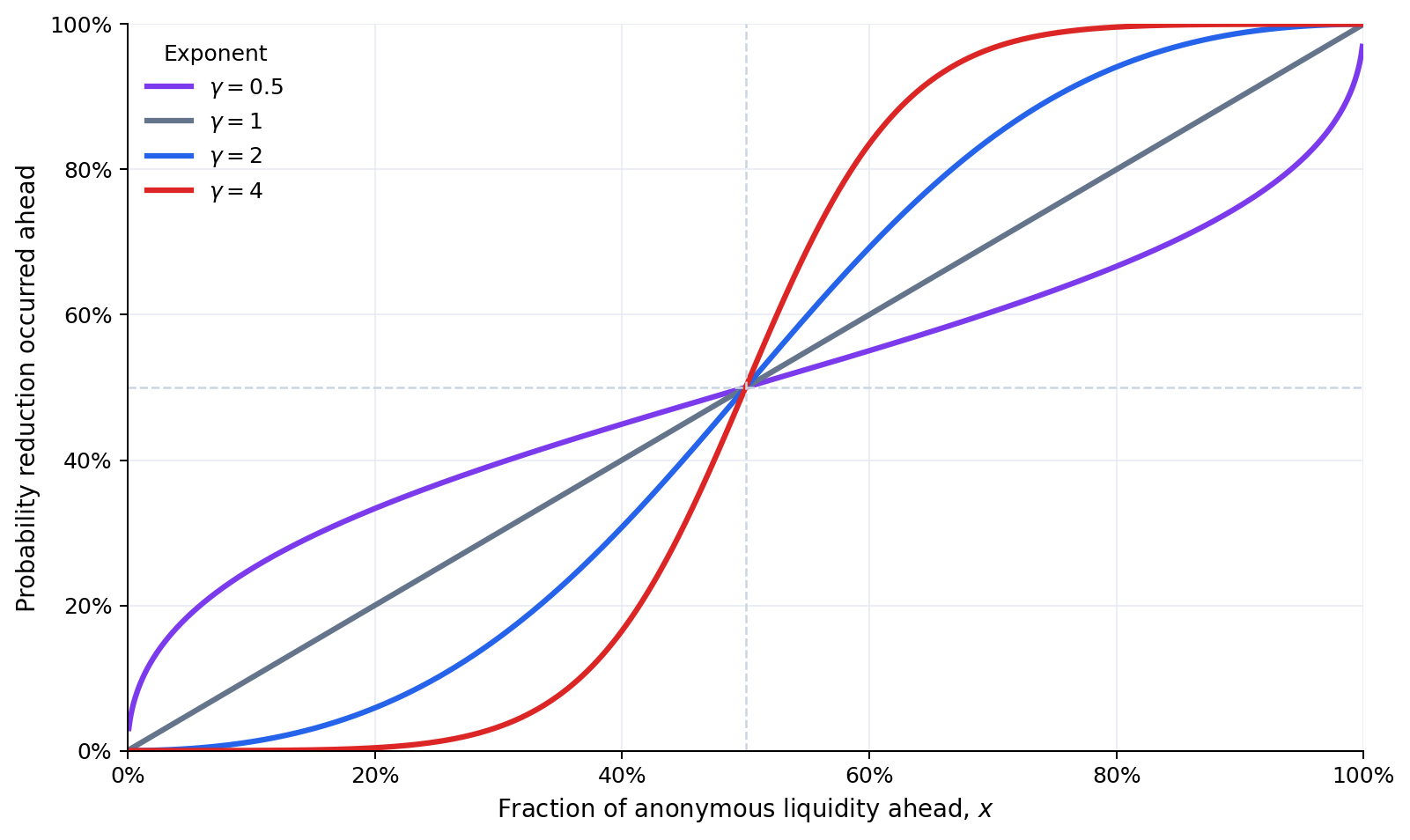
All curves meet at x=0.5. When the anonymous quantity is split equally ahead of and behind our order, the model assigns equal cancellation probability to both sides regardless of γ.

For γ > 1, the curve becomes steeper around the midpoint. The model increasingly assigns the reduction to whichever side contains more liquidity.

For 0 <γ < 1, the curve flattens. Cancellation probabilities are pulled towards 0.5, making the model less sensitive to the relative amount of liquidity ahead and behind us.

In practice, the probability function depends on rather predictable factors such as distance from the top of book. We can generalize the probability function by fitting different curves across reasonable market variables.

These policy choices and parameters can then be calibrated against empirical order traces.

Calibrating Queue Policies and Parameters

We now have several defensible impact and queue models. The remaining question is which model best represents the market we are trying to simulate.

Calibrating directly against strategy PnL is problematic. Market-making strategies are state-dependent: one different fill changes inventory, which changes subsequent quotes, cancellations and order sizes.

The action paths quickly diverge, leaving us unable to determine whether a PnL difference came from the queue model or from the strategy.

Instead, we calibrate through a closed-action replay. We hold the live order actions fixed and allow only their simulated outcomes to change.

Trace and tick-data objects

Event journalling architecture in quantpylib was discussed here:

HFT - Event Journaling and Quantpylib's Native Journaling Architecture

Consider an order trace containing:

• order and cancellation intents;

• submission and cancellation timestamps;

• side, price, size, order type and time-in-force;

• acknowledgements and terminal order states;

• fills, including their quantity, price and exchange timestamp.

From this trace, we may extract the exogenous action tape:

submit order A at t1
submit order B at t2
cancel order A at t3
submit order C at t4
...

The second object is the public tick-data stream. It contains the market events required to reconstruct exchange-side state:

Designing Institutional Data Capture for Quantitative Research.

• L2 snapshots and updates;

• trades;

• exchange and receive timestamps;

• …
  

The market data capture infrastructure in QuantPylib supports these artefacts.

For a candidate model θ, we replay the same action tape of order submissions and cancellations against the same tick-data stream.

In QuantPylib, the wall clock is swapped against the replay clock and the same trace architecture generates replay trace files. We can then compare the live trace fill against the simulated trace file in a queue replay harness.

We can therefore compare outcomes order by order and determine quantitatively the “fitness function of a queue model”.

Fill classification

Let I be the set of submitted order intents. Define:

\(F=\{i\in I:q_i>0\}\)

as the set of orders which received at least one live fill, and:

\(\widehat{F}_\theta = \{i\in I:\widehat{q}_{i,\theta}>0\}\)

as the set filled under candidate model θ.

Fill precision is:

\(P_\theta = \frac{|F\cap\widehat{F}_\theta|} {|\widehat{F}_\theta|}\)

This answers: when the simulation produces a fill, how often did that order also fill live?

Fill recall is:

\(R_\theta = \frac{|F\cap\widehat{F}_\theta|} {|F|}\)

This answers: how many live-filled orders did the simulation reproduce?

A combined F1 score is:

\(F_{1,\theta} = \frac{2P_\theta R_\theta} {P_\theta+R_\theta}\)

A pessimistic model may have excellent precision while missing many live fills. An optimistic model may reproduce most live fills while inventing many others.

Lifecycle accuracy

Let s_i and ŝ_i,θ be the terminal live and simulated states of order i, such as filled, partially filled, cancelled or rejected.

Lifecycle accuracy is:

\(A_{\text{status},\theta} = \frac{1}{|I|} \sum_{i\in I} \mathbf{1} \left[ s_i=\widehat{s}_{i,\theta} \right]\)

This catches differences which a binary filled/unfilled label misses, particularly partial fills and cancellation outcomes.

Fill timing

For orders filled in both traces, let t_i and t̂_i,θ be the timestamps of the first live and simulated fills. Define:

\(C_\theta=F\cap\widehat{F}_\theta\)

A smooth timing score is:

\(S_{t,\theta} = \frac{1}{|C_\theta|} \sum_{i\in C_\theta} \exp \left( -\frac{ |t_i-\widehat{t}_{i,\theta}| }{\tau} \right)\)

The scale τ determines the timing tolerance. The score ranges from zero to one. A score of one represents identical first-fill timestamps, while values near zero indicate timing errors which are large relative to τ. Semantically, it quantifies how closely the simulated trace reproduces first-fill timing for orders filled in both traces.

Fill-price similarity

Let p_i and p̂_i,θ be the live and simulated volume-weighted fill prices for an order filled in both traces.

The price error in basis points is:

\(e_{i,\theta} = 10^4 \frac{ |p_i-\widehat{p}_{i,\theta}| }{p_i}\)

We can convert this into a bounded score:

\(S_{p,\theta} = \frac{ \sum_{i\in C_\theta} w_i \exp \left( -\frac{e_{i,\theta}}{\kappa} \right) }{ \sum_{i\in C_\theta}w_i }\)

where κ controls the price-error tolerance and:

\(w_i = \min(q_i,\widehat{q}_{i,\theta})p_i\)

weights the comparison by overlapping filled notional.

For passive single-price orders, this metric may carry little information: both traces often fill at the submitted limit price. It is more useful for aggressive orders, multi-level executions and partial fills across prices.

Cancellation races

Cancellation behaviour deserves its own comparison. Let:

\(r_i = \mathbf{1} \left[ t_i^{\text{cancel intent}} < t_i^{\text{fill}} < t_i^{\text{cancel effective}} \right]\)

indicate that order i filled while its cancellation was in flight. Define r̂_i,θ similarly for the simulation. Cancellation-race accuracy is:

\(A_{\text{cancel},\theta} = \frac{1}{|I_{\text{cancel}}|} \sum_{i\in I_{\text{cancel}}} \mathbf{1} \left[ r_i=\widehat{r}_{i,\theta} \right]\)

This exposes a common source of optimistic replay: allowing the order to disappear when the strategy decides to cancel rather than when the cancellation reaches the exchange.

Trace similarity as a fitness function

The component metrics can be combined into a trace-similarity score:

\(S(\theta) = w_fF_{1,\theta} + w_sA_{\text{status},\theta} + w_qS_{q,\theta} + w_tS_{t,\theta} + w_pS_{p,\theta} + w_cA_{\text{cancel},\theta}\)

with:

\(\sum_j w_j=1\)

The weights should reflect the use case.

For calibration sessions D_train, we select:

\(\theta^\star = \arg\max_{\theta} \frac{1}{|\mathcal{D}_{\text{train}}|} \sum_{d\in\mathcal{D}_{\text{train}}} S_d(\theta)\)

The purpose is not to find the queue model which produces the highest backtest PnL. It is to find the model whose order-level outcomes most closely resemble the empirical trace.

thanks for reading. cheers!